Temporal Analysis with Stream Windowing Functions in DuckDB
Petrica Leuca, Gábor Szárnyas
Introduction
In data platforms, we usually categorize the data into dimension and fact data. While dimensions contain information about entities (name, address, serial number, etc.), facts contain events related to such entities (clicks, sales, bank transactions, readings from IoT devices, etc.). In general, fact data includes a timestamp attribute, denoting the moment when the event happened (or was observed).
When the timestamped data is processed on a streaming platform, it is often processed with stream windowing functions in order to organize the data into time windows.
In this post, we will show how to apply stream windows on static timestamped fact data in DuckDB, as part of a data analysis task to compute train service summaries, trends and interruptions at Amsterdam Centraal Station.
In a future post, we’ll cover streaming design patterns with DuckDB.
Warning The database is rather big (approx. 1.2 GB), therefore make sure to have a stable internet connection. Instead of attaching the database, you can also download the database file and connect to it from the command line:
Tumbling windows are fixed-size [left-closed, right-open) time intervals, used to calculate summaries at a certain time unit level (year, day, hour, etc.). Tumbling windows are also used to transform (irregular) fact data into time series data, by aggregating it at a regular time interval.
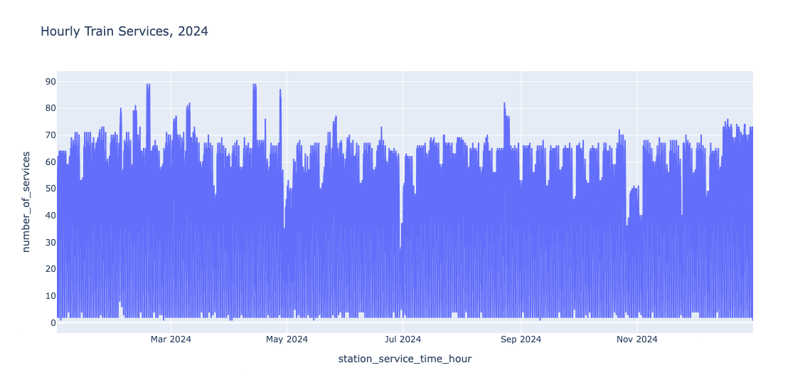
One way of implementing tumbling windows is to use the date_trunc function, which will truncate the timestamp to the specified precision. For example, in the following, we retrieve the number of services for each hour and each day in 2024:
SELECT
date_trunc('hour', station_service_time) AS window_start,
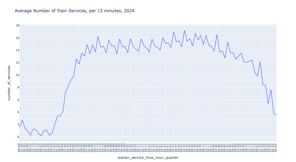
Another approach is to use the time_bucket function, which will truncate the timestamp to the bucket width provided, starting from the specified offset. For example, we calculate the number of services each quarter of an hour, starting with 00:
The time bucket function is generating the buckets from the timestamp column itself, there could be gaps in the time series data.
As seen in the above result, the first record is 2024-01-01 01:30:00, because there are no records before that timestamp.
Given that tumbling windows are non-overlapping intervals, we can calculate summaries, such as the average number of services during a 15 minute interval. It is interesting to observe that the number of train services is quite stable during the day but it’s much lower during the night – even in Amsterdam.
Hopping Windows
Hopping windows are fixed-size time intervals, but, contrary to tumbling windows, are overlapping. A hopping window is defined by:
how much time should elapse between the window start time, called hopping size;
how much time should a window contain, called window size.
One use case for hopping windows is to identify the five busiest 15-minute periods (window size) during 2024, starting every 5 minutes (hopping size). We start by generating artificial hopping windows for all the dates we are interested in:
WITH time_range AS (
SELECT
rangeAS window_start,
window_start + INTERVAL 15MINUTEAS window_end
FROMrange(
'2024-01-01 00:00:00'::TIMESTAMP,
'2025-01-01 00:00:00'::TIMESTAMP,
INTERVAL 5MINUTE-- hopping size
)
)
┌─────────────────────┬─────────────────────┐
│ window_start │ window_end │
│ timestamp │ timestamp │
├─────────────────────┼─────────────────────┤
│ 2024-01-01 00:00:00 │ 2024-01-01 00:15:00 │
│ 2024-01-01 00:05:00 │ 2024-01-01 00:20:00 │
│ 2024-01-01 00:10:00 │ 2024-01-01 00:25:00 │
│ · │ · │
│ · │ · │
│ · │ · │
│ 2024-12-31 23:45:00 │ 2025-01-01 00:00:00 │
│ 2024-12-31 23:50:00 │ 2025-01-01 00:05:00 │
│ 2024-12-31 23:55:00 │ 2025-01-01 00:10:00 │
├─────────────────────┴─────────────────────┤
│ 105408 rows (6 shown) 2 columns │
└───────────────────────────────────────────┘
We then join the above intervals with the train service data in order to calculate the number of services for each [left-closed, right-open) interval:
Can you imagine how it must have been like in the control room when within 15 minutes, 28 trains were arriving or departing in a station with 15 tracks?
By applying a RIGHT OUTER JOIN in the above query, gaps are filled with 0 number of services.
Sliding Windows
Sliding windows are overlapping intervals, but, compared to hopping windows, they are dynamically generated from the time column analyzed, therefore changing when new records are inserted.
Sliding windows can be implemented by using the RANGE window framing:
Because the current row is included in the calculation, the sliding windows are [left-closed, right-closed].
Session Windows
A session window groups events that happen close together in time, separated by inactivity gaps. A new session starts when the time between two events exceeds a defined timeout. The most common use case of session windows is to detect gaps in the timestamped data.
We continue the data analysis by identifying the days in which there were periods of time larger than 10 minutes in which no train was arriving/departing in/from the Amsterdam Centraal Station. In this context, a session window is the period of time in which train services run without a service inactivity gap longer than 10 minutes.
We start by calculating, for each record, the previous service time, by using the lag window function. We observed above that there is almost no traffic during the night, therefore we include only services between 6 AM and 11 PM:
SELECT
service_sk,
station_service_time,
lag(station_service_time) OVER (
PARTITIONBY station_service_time::DATE
ORDER BY station_service_time
) AS previous_service_time,
date_diff('minute', previous_service_time, station_service_time) AS gap_minutes
FROM ams_traffic_v
WHEREhour(station_service_time) BETWEEN6AND23
In the above query we also calculate the gap, in minutes, between the current service and the previous service, with date_diff. If there is no previous service, the column will be NULL, depicting the first service session in the day:
Tip Because gap_minutes is computed based on a window function, we can filter on it with QUALIFY, e.g.: QUALIFY gap_minutes IS NULL
We then mark if the current record is in the same session as the previous one, by comparing the minutes elapsed to a timeout, in our case 10 minutes:
IF(gap_minutes >=10OR gap_minutes ISNULL, 1, 0) AS new_session
By applying a moving sum, at day level, over the new_session attribute, we assign an identifier to the session:
sum(new_session) OVER (
PARTITIONBY station_service_date
ORDER BY station_service_time ROWSUNBOUNDEDPRECEDING
) AS session_id_in_day
Bringing it all together, we can now retrieve the dates which had at least one inactivity gap of 10 minutes during the 18 hours day service time (the number of hours between 6 AM and 11 PM):
WITH ams_daily_traffic AS (
SELECT
service_sk,
station_service_time,
lag(station_service_time) OVER (
PARTITIONBY station_service_time::DATE
ORDER BY station_service_time
) AS previous_service_time,
date_diff('minute', previous_service_time, station_service_time) AS gap_minutes
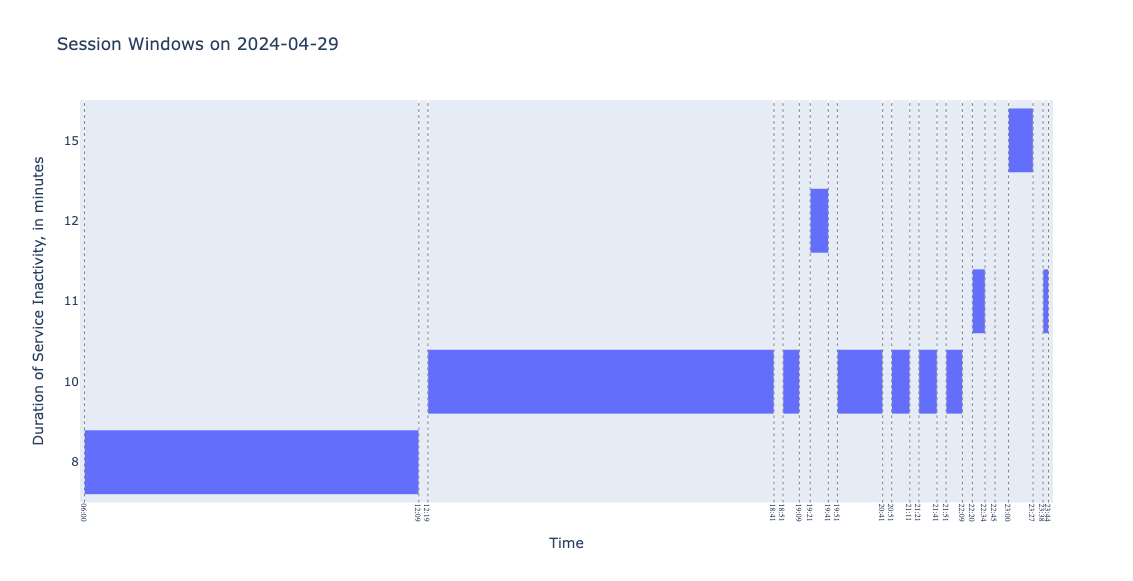
Something must have happened on 29 April 2024! We observe that, during the 18 hours of service, there were 12 session windows, which means that, for at least 10 times, no train arrived or departed during a period of 10 minutes. A reason for this could be that a regular train service was not running on that day. And indeed maintenance work started between Amsterdam and Utrecht.
In this post we have demonstrated how stream windowing functions can be implemented on historical timestamped data in DuckDB, offering a starting point in time (series) data analysis. We also recommend “Catching up with Windowing”, a post about DuckDB’s windowing features, which can be adopted in the functions presented herein.